Why Industrial IoT Data Breaks Traditional Databases

A production line reports temperature, vibration, spindle speed, and tool wear every 100 milliseconds. Three months in, the team adds coolant pressure sensors. Six months in, a new machine model arrives with a different payload format and different metric names. The schema designed on day one is wrong by month six, and maintaining it has become a recurring engineering task that competes with everything else on the backlog.

This is the normal lifecycle of industrial sensor deployments. And it exposes a gap that goes deeper than schema management: traditional databases were designed for transactional workloads with defined schemas, moderate write rates, and queries that return individual records by primary key. Industrial IoT data violates all three assumptions simultaneously.

The velocity problem: writes that never stop

Industrial environments write data continuously. ABB's industrial AI product Ability Genix ingests 1 million sensor values per second into CrateDB, while simultaneously retrieving 30,000 to 120,000 events per second for downstream AI workloads. SPGo processes 760 million records per day from sensor arrays at mining operations.

Traditional relational databases handle increasing write loads by doing more of what they were designed for: maintaining more indexes, managing more lock contention, sustaining more I/O. Under extreme write rates, that approach reaches its architectural limits. Index maintenance overhead slows ingestion during peak loads. Lock contention between concurrent writes and analytical reads creates query latency spikes exactly when the operations team is watching dashboards most closely.

CrateDB uses a shared-nothing distributed architecture where ingestion is spread across nodes from the start. Each node handles a share of the write load. Adding nodes adds ingestion capacity linearly. There is no primary node that absorbs all writes and becomes the bottleneck as volume grows.

Industrial telemetry is also append-heavy. Records are written and rarely updated. Traditional relational databases were built for a different pattern: moderate inserts with frequent updates. Columnar storage, where data is organized by column rather than by row, is a better fit for append-heavy analytical workloads. Writes are faster, compression ratios are higher, and analytical queries that scan a column across millions of records read far less data than row-oriented storage requires.

The schema problem: sensors change, schemas should too

Industrial sensor payloads rarely stay static. A firmware update adds new measurement fields. A machine from a new supplier uses different metric names. A plant expansion introduces sensor types that did not exist when the schema was first designed.

In a traditional relational database, each of these changes requires an ALTER TABLE statement. At scale, schema migrations compete with production write loads. Teams end up scheduling schema changes as production incidents, or running dual-write pipelines to keep old and new formats compatible in parallel.

InfluxDB's tags and fields model imposes a similar constraint at a different layer. Tags define the identity of a series; fields hold the measurements. The model assumes you know your sensor schema in advance and that tag combinations are bounded. Adding a measurement type that introduces new tag combinations means revisiting the data model at design time, not just writing a new record. For a full comparison of how the architectures handle this, see CrateDB vs InfluxDB: IoT Time-Series Database Comparison.

CrateDB handles this through dynamic columns. Declare a column as OBJECT(DYNAMIC) and any field in an incoming JSON payload that does not match a declared column is stored automatically, indexed immediately, and queryable in standard SQL from the next statement onward. 

-- Define a table with a dynamic column for sensor readings
CREATE TABLE sensor_readings (
    ts        TIMESTAMP WITH TIME ZONE,
    asset_id  TEXT,
    readings  OBJECT(DYNAMIC)
) CLUSTERED BY (asset_id);

-- A new sensor type writes its first record.
-- coolant_pressure_bar did not exist in the original schema.
INSERT INTO sensor_readings (ts, asset_id, readings)
VALUES (
    NOW(),
    'cnc-line-04',
    '{"temperature_c": 82.3, "coolant_pressure_bar": 4.1}'
);
-- CrateDB indexes coolant_pressure_bar immediately. No ALTER TABLE required.

For a step-by-step walkthrough of adding a new sensor type to a live deployment without stopping ingestion, see How to Add a New Sensor Type to Your Industrial Database Without Pipeline Downtime.

Rauch Group processes 400 data records per second across food manufacturing lines with varying sensor configurations. When a new sensor type comes online, the ingestion pipeline does not change. The field arrives. CrateDB indexes it. The operations team queries it.

The cardinality problem: the ceiling that arrives without warning

High cardinality means a large number of unique values in a dimension. In industrial data, cardinality is structural. Every device has a unique identifier. Every facility has a code. Every production batch has a number. A deployment with 10,000 devices across 50 facilities using 20 sensor types per device has 10 million potential unique identifier combinations, before adding firmware version, operating mode, or customer tenant as further dimensions.

InfluxDB creates one time series per unique combination of tag values. Each series gets an entry in an in-memory index. At low cardinality this index is small and fast. As device fleets grow, the index grows proportionally. At high enough cardinality, the index exhausts available memory. Write performance degrades as new series entries require index expansion. Query performance degrades as the index becomes a bottleneck in the read path.

This is not a misconfiguration. It is the documented architectural cost of the series-per-tag-set design, and why high-cardinality workloads — large device fleets, per-user time series, per-session metrics — are cases where this constraint becomes a hard limit. For a detailed breakdown of how the cardinality architectures differ, see The InfluxDB Cardinality Problem: Why High-Cardinality Industrial Data Breaks It. For how high cardinality fits into a broader architecture covering JSON schema evolution, observability, and mixed workloads, see Beyond Time-Series: High-Cardinality Analytics, Flexible JSON, and Unified Observability.

TGW Logistics manages 900,000 sensors per distribution center. At that scale, a database whose performance degrades with cardinality does not present a tuning challenge. It forecloses the deployment architecture entirely.

CrateDB uses a columnar architecture with no per-series in-memory index. Every field in every record is indexed at ingestion using columnar inverted indexes, regardless of how many unique values that field contains. Adding a device to a fleet of 100,000 is the same operation as adding a device to a fleet of 10. Query performance across 900,000 sensors does not degrade as the fleet grows because the query path does not depend on an in-memory series count.

The query problem: time-series, search, and analytics in one engine

Industrial analytics is not a single query type. Operational teams need aggregations across billions of sensor events, anomaly detection over recent time windows, correlation between assets on the same production line, full-text search across maintenance logs, and geospatial queries against mobile assets — often in the same dashboard, in the same shift.

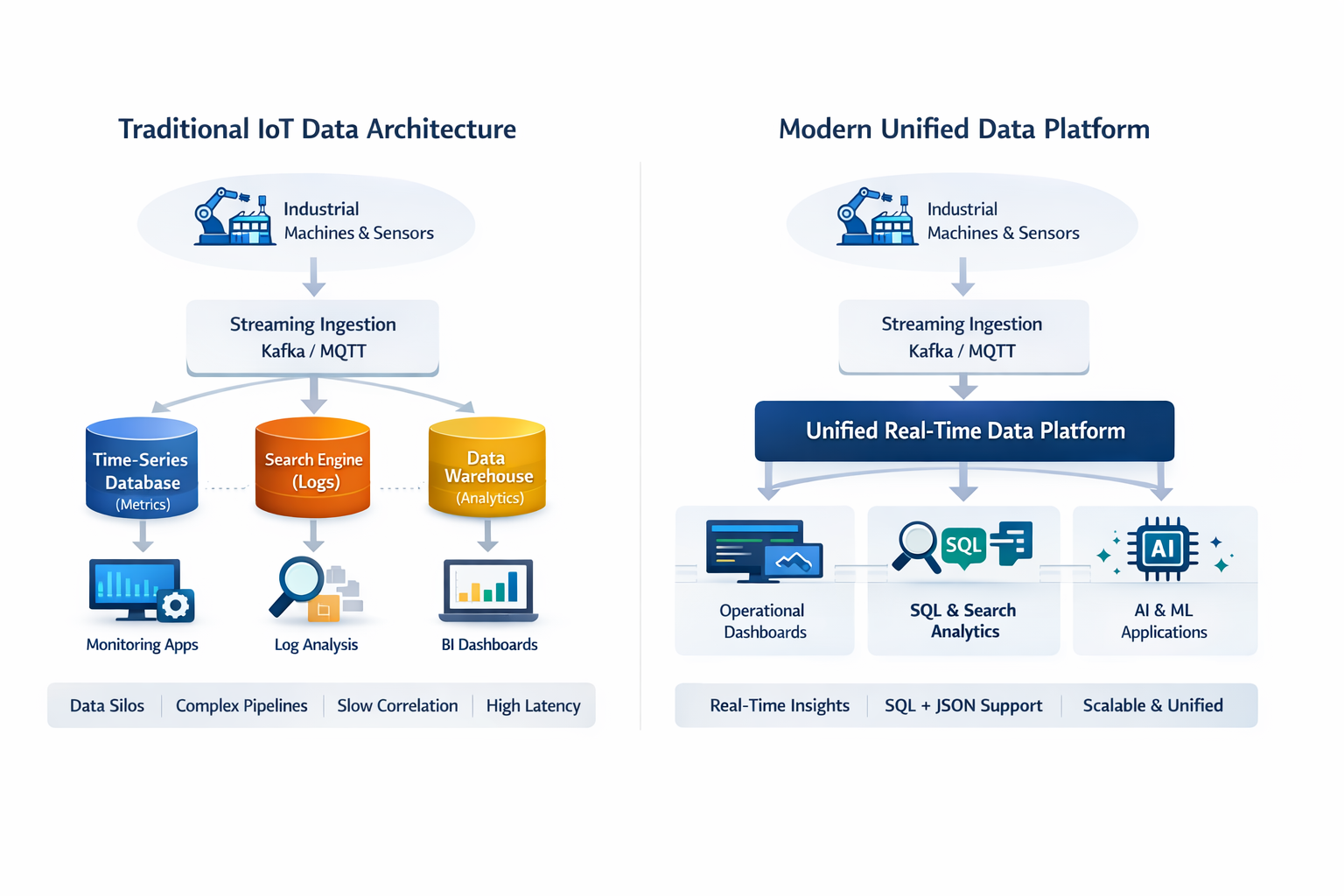
Traditional architectures handle this by splitting the workload across specialized systems: a time-series database for metrics, a search engine for maintenance logs, a relational system for production events, a data warehouse for historical aggregations. Each system solves one problem well. But keeping them synchronized, managing four query languages, and debugging failures across the boundaries between them is an ongoing engineering cost that compounds as the analytics requirements grow.

CrateDB stores time-series, JSON, full-text, and relational data in the same engine and queries all of it in standard SQL. A single query can join a sensor reading from the last 10 minutes with a full-text search across maintenance notes for the same asset:

-- Find assets with recent vibration anomalies that also have open bearing-related maintenance notes
SELECT
    s.asset_id,
    MAX(s.vibration_rms_ms2)  AS peak_vibration,
    m.note_text               AS maintenance_note,
    m.created_ts              AS note_created
FROM sensor_readings  s
JOIN maintenance_logs m ON s.asset_id = m.asset_id
WHERE s.ts > NOW() - INTERVAL '10 minutes'
  AND s.vibration_rms_ms2 > 4.5
  AND MATCH(m.note_text, 'bearing')
GROUP BY s.asset_id, m.note_text, m.created_ts
ORDER BY peak_vibration DESC;

That query correlates a real-time sensor anomaly with a free-text maintenance record. It runs against data that was indexed milliseconds ago, in a single statement, with no external search index to synchronize. There is no second system. There is no pipeline keeping the sensor store and the log store in sync.

OEE is a concrete example of the same principle at the production level. Calculating Availability, Performance, and Quality simultaneously requires joining downtime event records, cycle time sensor readings, and inspection logs. Traditional architectures put each of those in a separate store. In CrateDB they join in SQL against live data, and the dashboard reflects the current shift rather than last night's export. For the full OEE architecture, see OEE Analytics on Live Data: How to Move from Nightly Exports to Real-Time Dashboards.

The time problem: data arrives, queries should work immediately

Batch-oriented analytics systems require a load step. Data lands in a staging area, a pipeline moves it, indexes are updated, and only then does the data become queryable. That cycle takes minutes. In industrial operations, minutes cost money.

A vibration anomaly that triggers a maintenance alert needs to be detectable the moment it occurs, not after the next pipeline run. A packaging machine drifting out of spec needs to appear on the quality dashboard before an entire batch is written off. An OEE figure should reflect the floor state as of the last sensor reading, not last night's export.

CrateDB indexes every field on ingestion, in milliseconds. A sensor reading written to the database is in the next query's result set. There is no wait state between ingest and query. When ABB's Ability Genix retrieves 30,000 to 120,000 events per second for industrial AI inference, those events are fresh. The predictive maintenance model is running against data that arrived seconds ago, not minutes.

Five constraints, one architecture decision

These five problems do not arrive one at a time. A new industrial IoT deployment hits all of them within the first year: velocity as the device fleet scales, schema drift as firmware updates arrive, cardinality as device IDs multiply, query complexity as dashboards add dimensions, and freshness requirements as operations teams start acting on the data in real time.

A database architecture that handles four of these five and fails on the fifth still requires a workaround. That workaround becomes a second system, a synchronization pipeline, a schema migration window, or an engineering team dedicated to keeping the stack running. The cost compounds over time.

CrateDB customers in industrial and IoT deployments are running all five constraints simultaneously in production:

• ABB's Ability Genix ingests 1 million sensor values per second and retrieves 30,000 to 120,000 events per second for industrial AI workloads.
• TGW Logistics queries 900,000 sensors per distribution center to power real-time operational analytics and digital twin models.
• SPGo processes 760 million records per day from 30,000 sensors per mine for predictive maintenance analytics.
• Rauch Group processes 400 data records per second across food manufacturing lines with varying sensor configurations.

All four run the same SQL on the same distributed engine: no pre-aggregation step, no schema migrations for new sensor types, no cardinality ceiling, and no batch pipeline between ingest and query.

Before committing to an architecture, Comparing MongoDB, TimescaleDB, InfluxDB, and CrateDB for Industrial IoT maps how each option handles the five constraints described above. You can also Run queries against a live industrial dataset.