In this tutorial, we'll explore how you can leverage CrateDB as as time-series database and what you can do with your Free tier cluster. Using the sample dataset from the public records from taxi services in New York City you can learn how CrateDB Cloud makes it easy to explore time-series data in different ways while obtaining fast results. No prior SQL knowledge is needed.
The only knowledge you need is being able to access the console for the Free tier cluster you created. (If you have forgotten how to do so, take another look at the end of our Free tier guide.) Everything in this quick guide will be done in that console, or the CrateDB Admin UI, an easy-to-use interface that makes running queries fast and straightforward.
Now that you have some data ready, let’s look at some of the things you can do with CrateDB Cloud. First off, you do not need to wait for the data import to finish. It runs as a background process and will take some time, but you can already start playing around with the data as it is being imported.
When the data is fully imported, you will have about 6.3 Million data records in your cluster and about 94 MB of data. A decent size dataset to start with. In fact, CrateDB Cloud is built to handle queries on terabytes of data at great speed - but waiting to import that much would take too long for a quick showcase. With our NYC taxi sample dataset you don't have wait for long when you want to get started right now!
The dataset you'll be working with contains a collection of various bits of information about taxi trips taken by people in New York City. Beginning with the basics, you'll see how to load that data and how to manipulate it in various ways to retrieve particularly interesting subsets of the total information available.
You'll want to look at the dataset as a whole first. Running:
SHOW CREATE TABLE nyc_taxi;
will print what the table looks like:
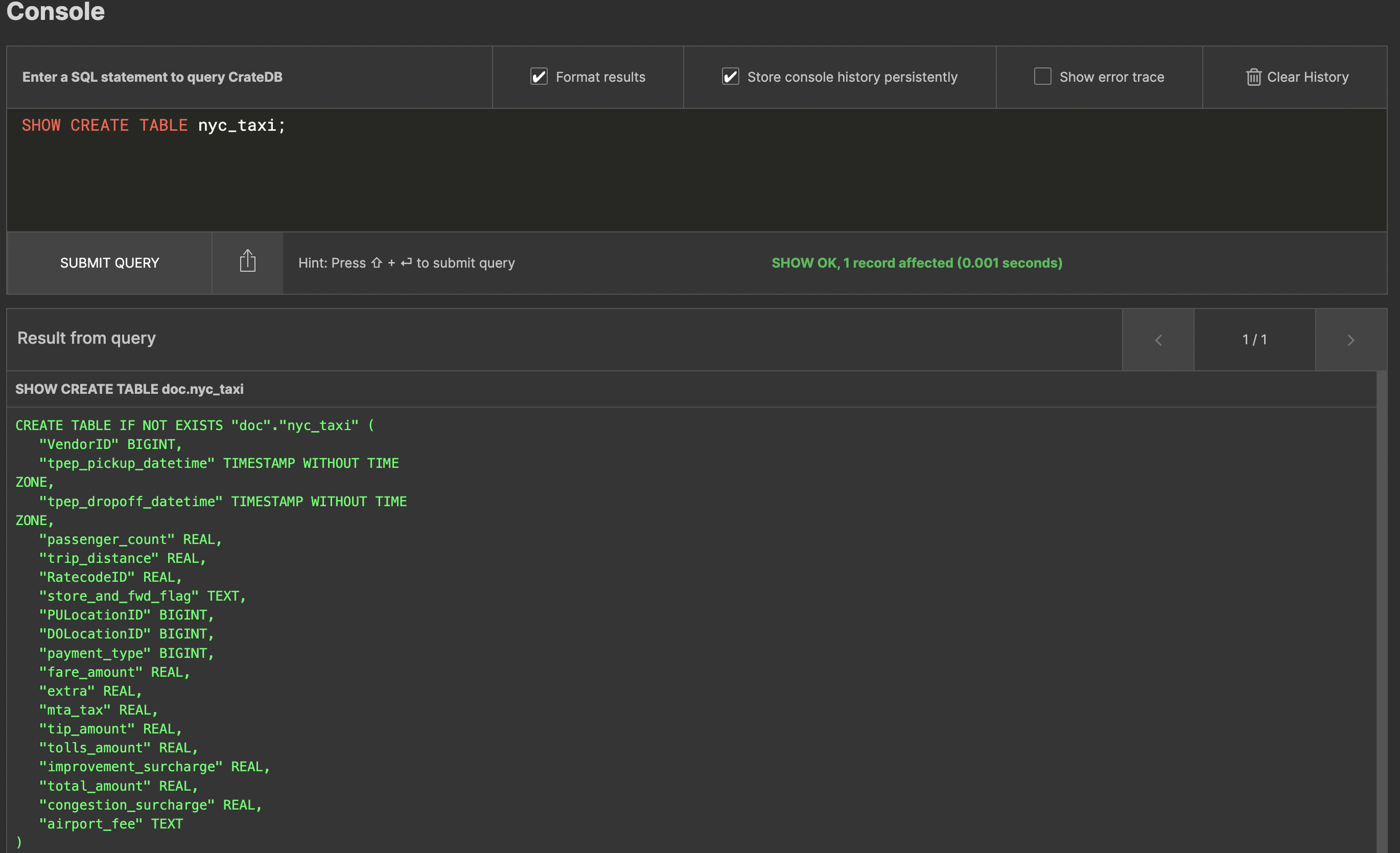
You have quite a bit of information about each journey: fare amounts, passenger numbers, tips and tolls paid... so what can you do with all that?
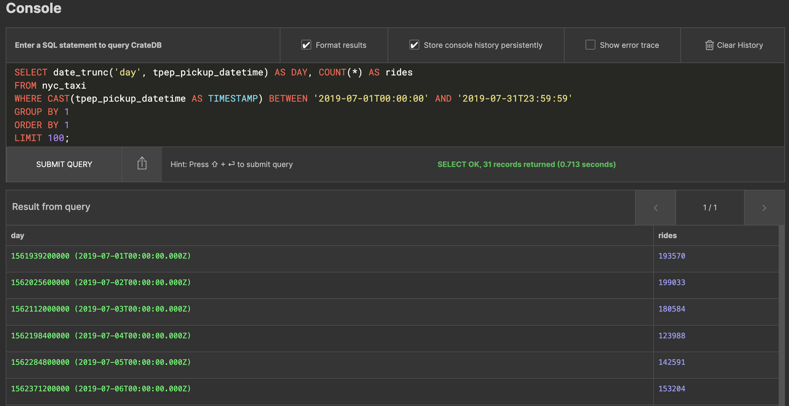
Let’s say you want to get the stats of how many rides there were per day during July of 2019. You can easily do that with a query like:
SELECT date_trunc('day', tpep_pickup_datetime) AS day, COUNT(*) AS rides
FROM nyc_taxi
WHERE CAST(tpep_pickup_datetime AS TIMESTAMP) BETWEEN '2019-07-01T00:00:00' AND '2019-07-31T23:59:59'
GROUP BY 1
ORDER BY 1
LIMIT 100;
This will look as follows:
Not a bad start. But it can get more interesting. Now let’s say you want to know the total distance travelled on any of those days, as well as the average distance per trip. You can do that too:SELECT date_trunc('day', tpep_pickup_datetime) AS DAY, COUNT(*) AS rides, SUM(trip_distance) AS total_distance, SUM(trip_distance) / COUNT(*) AS average_per_ride
FROM nyc_taxi
WHERE tpep_pickup_datetime BETWEEN '2019-07-01T00:00:00' AND '2019-07-31T23:59:59'
GROUP BY DAY
ORDER BY 1
LIMIT 100;
This gives you something a bit more interesting:
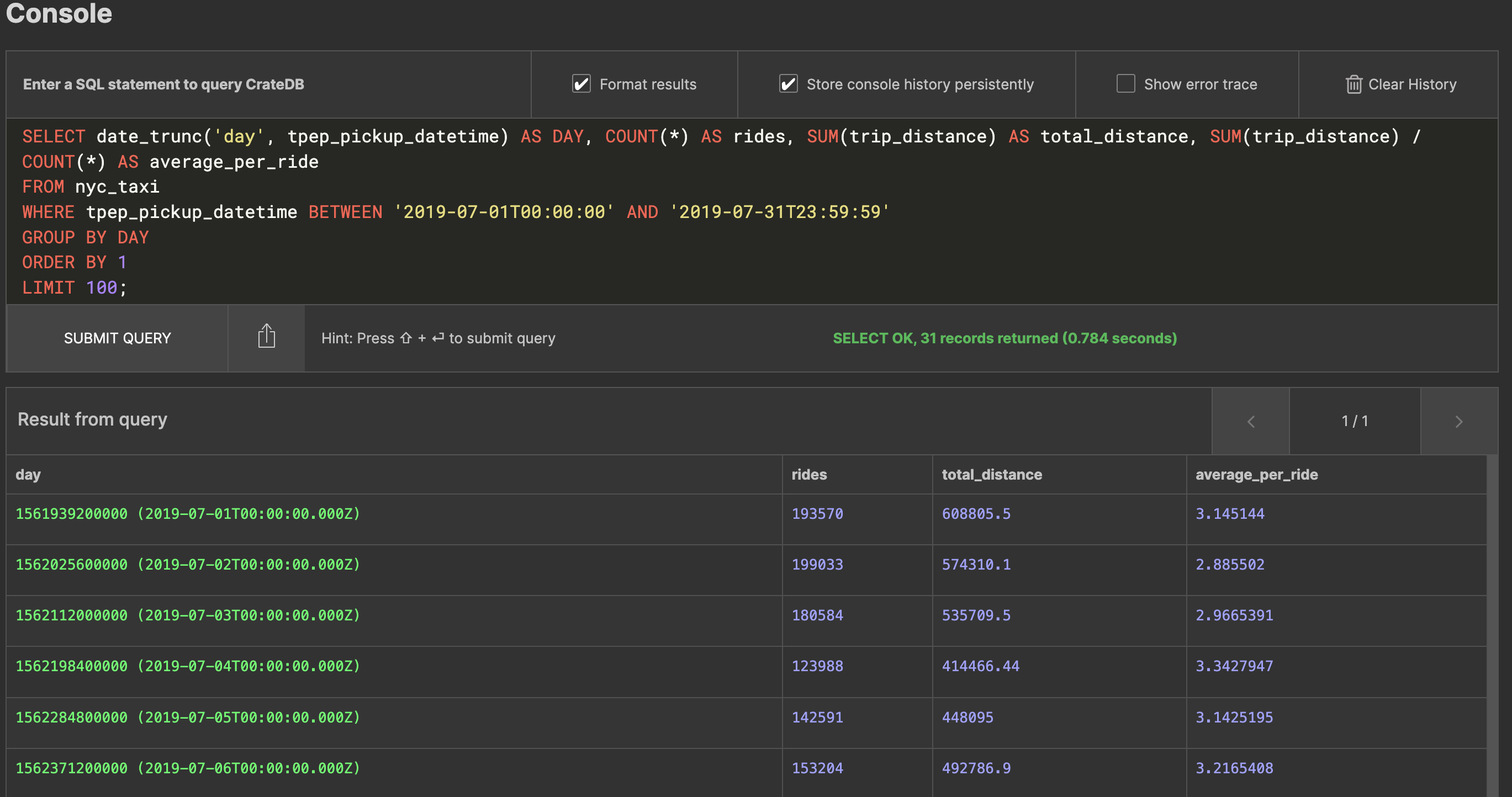
As you can now see from the dataset, when they take a cab New Yorkers go about 3 miles per trip on average.
Next, let’s say you want to figure out what the busiest hours of the day are. This, too, is easy enough to do:SELECT EXTRACT(HOUR FROM tpep_pickup_datetime) AS HOUR, COUNT(*), SUM(trip_distance) AS total_distance
FROM nyc_taxi
WHERE tpep_pickup_datetime BETWEEN '2019-07-01T00:00:00' AND '2019-07-31T23:59:59'
GROUP BY HOUR
ORDER BY COUNT(*) DESC
LIMIT 100;
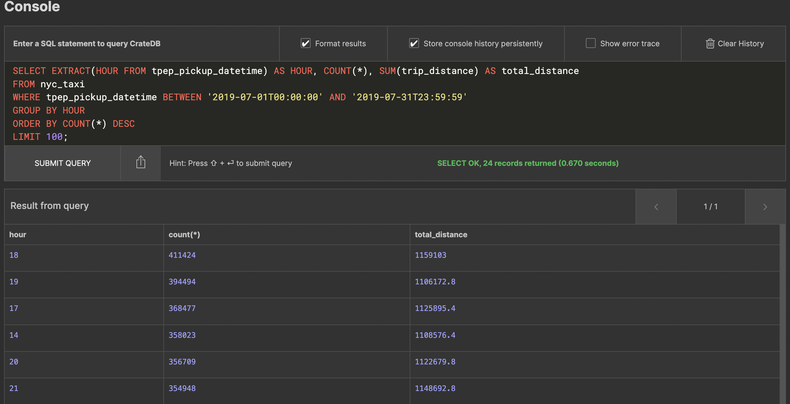
Unsurprisingly, New Yorkers tend to take the most taxi rides in the afternoon and after work at 6 PM.
So far it’s all been pretty standard SQL that you may be familiar with anyway. So, what can CrateDB Cloud really do? Let’s take a look at some more advanced possibilities and put it to the test.
You can load pretty large amounts of data into CrateDB Cloud: tens of terabytes are not a problem. The data is also compressed by default and all the fields are indexed – so you don’t need to worry about having to define indices in advance.
If you’ve ever worked with such large amounts of data, you will know that some queries can suddenly become quite tricky to handle. Let's say we want to get the number of unique pickup locations from the entire dataset – you would normally do something like a:
SELECT COUNT(DISTINCT(pulocationid)) FROM nyc_taxi;
Go ahead and try. You’ll see CrateDB Cloud immediately trip a circuit breaker – the amount of data is quite large, and CrateDB Cloud knows that it can’t reasonably perform this query without having to do a ridiculous full scan of the table.
Fortunately, there is a solution for that! It comes in the form of SELECT HYPERLOGLOG_DISTINCT(pulocationid) FROM nyc_taxi;
This uses an algorithm to estimate the number of data records, and is blazing fast, even on very large datasets:

You can use HYPERLOGLOG_DISTINCT() just like you can COUNT(DISTINCT) in any of your queries.
What about something really advanced? Imagine you want to get the list of the most high-grossing location pairs in NYC for the entire year. Not only that, but for each pair, you want to know how much more it grosses than the next best one. Here, window functions come to the rescue, which are well supported by CrateDB Cloud:
SELECT "PULocationID", "DOLocationID", cnt, total, next_highest_grossing, total - next_highest_grossing AS leads_by
FROM (
  SELECT
    "PULocationID",
    "DOLocationID",
    COUNT(*) AS cnt,
    SUM(total_amount) AS total,
    LAG(SUM(total_amount), 1) OVER (ORDER BY SUM(total_amount)) AS next_highest_grossing
  FROM nyc_taxi
  WHERE tpep_pickup_datetime BETWEEN '2019-01-01T00:00:00' AND '2019-12-31T23:59:59'
  GROUP BY "PULocationID", "DOLocationID"
  ORDER BY total DESC
  LIMIT 100
) AS sub;
In this case the query involves using the LAG() window function, which selects the next highest grossing amount from your list. The results look like this:
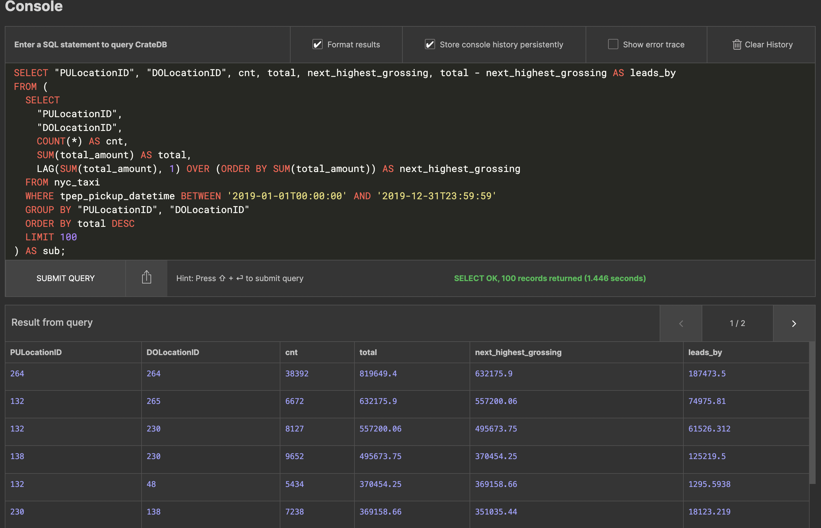
If you explore the results further, you may notice that 264 is a location called "Unknown". This just goes to show that no dataset is perfect... The second on the list is 132 to 230, which is JFK Airport to Times Square – we're not experts in NYC taxi patterns, but we're sure you'll agree that sounds plausible.
Of course, these are just some examples. Hopefully with this guide you have gotten an idea of some of the things you can do with your data in CrateDB Cloud. You can read up more about what queries are supported in CrateDB, our underlying database, in our official documentation. Finally, feel free to sign up for our Free tier cluster. This tier allows you to experiment with CrateDB Cloud for free on a single node with 2 CPUs, 2 GiB of memory and 8 GiB of storage.
In the meantime, have fun exploring the data with your CrateDB Cloud Free tier cluster. If you have any questions, feel free to reach out to us.


