We are thrilled to announce that in CrateDB version 5.6.0, we introduced a BKD-tree-based indexing strategy for geometric shapes. In this blog post, we delve into the significance of this addition. We explain how it enhances spatial indexing capabilities and accelerates performance of geospatial queries.

Introduction

CrateDB has long supported geometric shapes, facilitating the storage of various entities such as points, lines, and polygons. Leveraging these capabilities, developers can execute geospatial queries for equality, containment, intersection, and more.

To enhance query performance, specialized indexes are essential. Until recently, CrateDB exclusively offered an indexing strategy based on prefix trees, including two variants: one utilizing geohashes and the other employing quadtrees. In this method, the earth's surface is partitioned into grid layers, each layer possessing increasing precision. The top layer comprises a single grid cell, while lower layers consist of numerous cells covering equivalent spaces. Each grid cell, on every layer, is addressed in 2D space. Grid cell addresses share a common prefix between lower and upper layers, enabling their representation via a prefix tree. Geometric shapes are represented using these grid cells, as depicted in the example below:

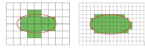
The two images illustrate an important property of this method. The size of a grid cell directly influences the accuracy of shape representation. Although smaller cells offer greater precision, they require more storage and lead to slower processing. While prefix tree-based indexes provide various configuration options, such as precision tuning, finding a sweet spot between spatial accuracy and query performance can sometimes be challenging. This task demands considerable effort and a deep understanding of internal data structures from users.

BKD-trees 

BKD-trees are multidimensional indexing structures designed to efficiently organize spatial data in a hierarchical manner. The key concept behind a BKD-tree is its ability to recursively partition data space along alternating dimensions. At each level of the tree, a split is made along one of the dimensions, dividing the data into two subsets. This process continues recursively until each subset contains a limited number of data points or until a specified depth is reached. The result is a hierarchical tree structure where each node represents a partition of the data space.

In CrateDB's indexing strategy based on BKD-trees, a geometric shape is decomposed into a collection of triangles. Each triangle is represented as a 7-dimensional point and stored in this format within a BKD-tree. To improve the storage efficiency of triangles within an index, the initial four dimensions are used to represent the bounding box of each triangle. These bounding boxes are stored in the internal nodes of the BKD-tree, while the remaining three dimensions are stored in the leaves to enable the reconstruction of the original triangles.

BKD-tree-based indexes in CrateDB

Let's now explore how we can practically utilize the new indexing method. If you're already familiar with CrateDB's geo search capabilities, you'll notice that the only difference between the new and previous approaches lies in how indexes are configured. However, if you're new to this topic, we provide a simple example in this section to demonstrate how to begin working with geometric shapes in CrateDB. We highly recommend exploring the topic of geo search further by referring to the more comprehensive documentation.

To create a table with a column of the geo_shape type, indexed using the BKD-tree-based strategy, you can simply define it as exemplified by the shape column below:

CREATE TABLE shapes (
  id integer primary key,
  shape geo_shape index using bkdtree
);

There's no need to include additional parameters like precision or tree levels, as required with other geospatial index types. The BKD-tree-based indexing strategy maintains the original shapes with an accuracy of 1 cm.

Next, we can insert shapes into our table:

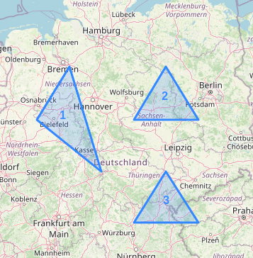
INSERT INTO shapes (id, shape) VALUES (1, 'POLYGON ((9 53, 8 52, 10 51, 9 53))');
INSERT INTO shapes (id, shape) VALUES (2, 'POLYGON ((12 53, 11 52, 13 52, 12 53))');
INSERT INTO shapes (id, shape) VALUES (3, 'POLYGON ((12 51, 11 50, 13 50, 12 51))');

These shapes can be depicted on the map in the following way:

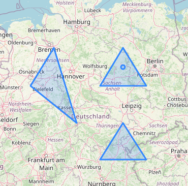
If, for example, we wish to determine which shapes contain the point (12, 52.5), we can execute the following query:

SELECT id FROM shapes WHERE match(shape, 'POINT(12 52.5)') USING intersects; 

It should return one row:

|  id |
| --- |
|  2  |

This result is correct, as shown on the map:

Now, if we would like to obtain reverse results, meaning all shapes that don’t contain the point, we can replace intersects with disjoint:

SELECT id FROM shapes WHERE match(shape, 'POINT(12 52.5)') USING disjoint; 

The results are as follows:

| id  |
| --- |
|  1  |
|  3  |

It's important to highlight that, as mentioned earlier, in BKD-tree-based indexes, shapes are preserved with an accuracy of 1 cm. While this precision is very high, if you find it insufficient, it may be worthwhile to consider using the prefix tree strategy instead.

Benchmarks

We ran a benchmark on a 3-node cluster. Each node had 4 AMD EPYC CPU cores and 2GB allocated for heap.

Our benchmark focused on two key aspects: indexing and lookup. To assess these, we created two simple tables having only geo_shape columns and executed multiple iterations of insert and select statements.

During the benchmark, the ratio of total execution time for INSERT queries between the prefix tree index and the BKD-tree index remained constant at around 3.0, regardless of the number of iterations: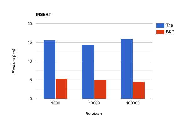

The total execution time ratio for SELECT queries between the prefix tree and BKD-tree indexes fluctuated between 2.5 and 3.5. With an increase in the number of iterations from 1000 to 10000, the BKD-tree-based index performed up to 3.5 times better. However, with further increases, the ratio dropped back to the initial 2.5:

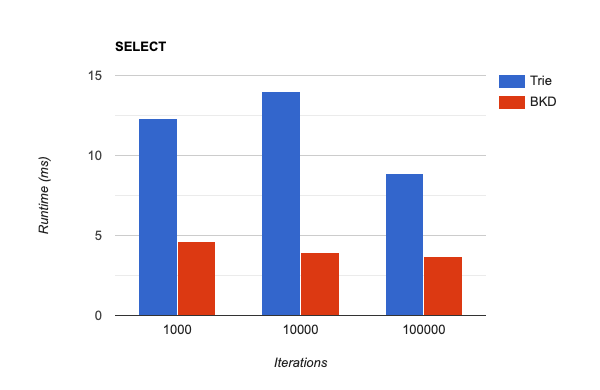
As shown above, in our benchmarks, the BKD-tree-based index outperformed the prefix tree-based index in both insertion and lookup operations. Indexing was approximately three times faster, and lookup was 2.5-3.5 times faster, depending on the input size.

Summary

This blog post highlights the challenges of balancing accuracy and performance in spatial data indexing. As we have seen, the introduction of BKD-tree-based indexing has brought notable enhancements in query performance (both indexing and lookup), streamlined index configuration and minimized storage demands. We believe that this update unlocks new possibilities for CrateDB users in spatial data exploration and analysis.