Time series decomposition is a statistical technique that helps with understanding the inherent patterns within time series data, such as identifying the long-term direction (trend), recurring patterns at fixed intervals (seasonality), and randomness (irregular fluctuations):
- Seasonality: The seasonal component captures regular patterns that repeat over fixed periods, such as daily, monthly, or quarterly fluctuations. Seasonality is influenced by various factors like weather, holidays, and business cycles.
- Trend: The trend component represents the long-term progression of the series, showing how the data moves up or down over a lengthy period. It's essentially the underlying direction in which the data is heading, excluding shorter-term fluctuations.
- Residual (Irregular Component): After the trend and seasonal components are removed from the original time series, the remainder is the residual component. It consists of irregular or random fluctuations that cannot be attributed to the trend or seasonal effects. This component can sometimes reveal unusual events or outliers not explained by the trend or seasonality.
Practical Application of Data Decomposition with PyCaret and CrateDB
Steps 1 to 6
To follow this tutorial, repeat Steps 1 through 6 from the explanation on Exploratory Data Analysis. Once the environment is set up, proceed to the next step for visualizing time series decomposition.
Step 7. Visualizing Time Series Decomposition
We employ PyCaret to automate the analytical process and visualize the time series decomposition.
import plotly

# Plotly plots will be rendered as PNG images, uncomment the following line to crate an interactive chart
plotly.io.renderers.default = 'png'
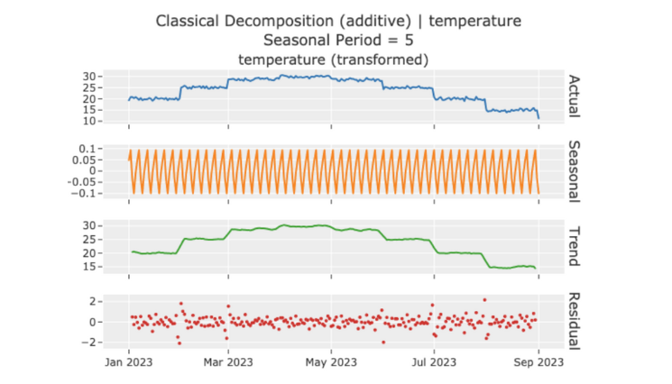
eda.plot_model(plot="decomp")
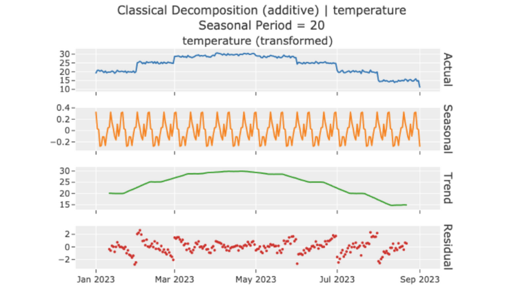
eda.plot_model(plot="decomp", data_kwargs={'seasonal_period': 20})
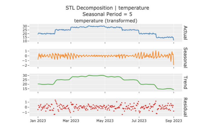
eda.plot_model(plot="decomp_stl")
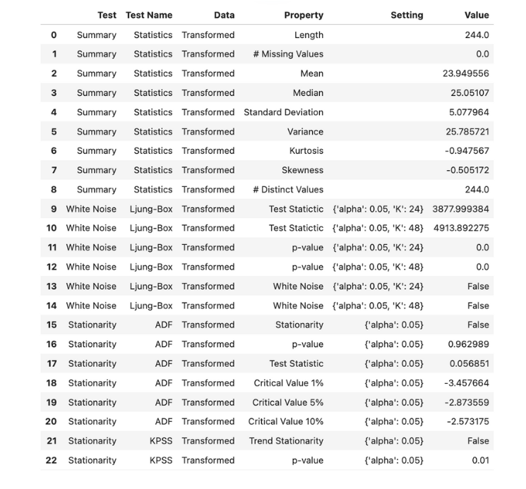
With this overview of time series decomposition with PyCaret and CrateDB, you now have a solid understanding of the data’s statistical properties which is essential for reliable and insightful anomaly detection and forecasting.
