Indexing and storage in CrateDB¶

Marija Selakovic

November 12, 2021

8 min read

Introduction¶

This article explores the internal workings of the storage layer in CrateDB. The storage layer ensures that data is stored in a safe and accurate way and returned completely and efficiently. CrateDB’s storage layer is based on Lucene indexes.

What’s inside¶

Lucene offers scalable and high-performance indexing, which enables efficient search and aggregations over documents and rapid updates to the existing documents. We will look at the three main Lucene structures that are used within CrateDB: Inverted indexes for text values, BKD trees for numeric values, and doc values.

Inverted index:: Understand how inverted indexes are implemented in Lucene and how CrateDB uses them to index text values and enable fast text searches.
BKD tree:: Understand the BKD tree, starting from KD trees, and how this data structure supports range queries on numeric values in CrateDB.
Doc values:: This data structure enables efficient queries by document field name, performs column-oriented retrieval of data, and improves the performance of aggregation and sorting operations.

Indexing text values¶

The Lucene indexing strategy relies on a data structure called inverted index. An inverted index is defined as a “data structure storing a mapping from content, such as words and numbers, to its location in the database file, document or set of documents“ [Wikipedia]. In Lucene, an index can store an arbitrary size of documents, with an arbitrary number of different fields.

To better explain how inverted indexes are implemented in Lucene, we first introduce Lucene Documents. A Lucene Document is a unit of information for search and indexing that contains a set of fields, where each field has a name and value. Furthermore, each field can be tokenized to create terms. We refer to terms as the smallest units of search and index and they are represented as a combination of a field name with a token. Depending on the analysis, generated terms dictate what type of search we can do efficiently and which not.

Finally, the Lucene index is implemented as a mapping from terms to documents and it is called inverted because it reverses the usual mapping of a document to the terms it contains. The inverted index provides an effective mechanism for scoring search results: if several search terms map to the same document, then that document is likely to be relevant.

Indexing is done before retrieval, and access is done on indexed documents. The major steps in the creation of the Lucene index are illustrated in the following example:

Imagine that we collected two documents to be indexed: “My favorite sweet dish is strawberry cake.“ and “Strawberries are bright red and sweet.“
The next step is the tokenization of text into words: “My“, “favorite“, “sweet“, “dish“, etc.
To produce indexing terms, we use linguistic processing for token normalization. For example, the term “Strawberries“ is normalized to “strawberry“ and the result is used as an indexing term.
Each indexing term is then mapped to document id and the resulting sequence of terms is sorted alphabetically. The instances of the same term are then grouped by word and by document id. The final index contains indexing terms and pointers to the posting lists, i.e., the list of document ids that hold the term.

The diagram below shows the indexing terms from two documents, the sorted sequence, and finally the index.

Indexing terms sorted sequence and index

Lucene segments¶

A Lucene index is composed of one or more sub-indexes. A sub-index is called a segment, it is immutable and built from a set of documents. When new documents are added to the existing index, they are added to the next segment. Previous segments are never modified. If the number of segments becomes too large, the system may decide to merge some segments and discard the corresponding documents. This way, adding a new document does not require rebuilding the index structure.

Inverted indexes¶

CrateDB splits tables into shards and replicas, meaning that tables are divided and distributed across the nodes of a cluster. Each shard in CrateDB is a Lucene index broken into segments and stored on the filesystem. Depending on the configuration of a column the index can be plain (default) or full-text. An index of type plain indexes content of one or more fields without analyzing and tokenizing their values into terms. To create a full-text index, the field value is first analyzed and based on the used analyzer, split into smaller units, such as individual words. A full-text index is then created for each text unit separately.

To illustrate both indexing methods, let’s consider a simple table called Product:

productID	name	quantity
1	Almond Milk	100
2	Almond Flour	200
3	Milk	300

The inverted index enables a very efficient search over textual data. For our case, it makes sense to index the column “name”. The next two tables illustrate the resulting plain and full-text indexes:

Plain index

name	docID
Almond Milk	1
Almond Flour	2
Milk	3

Fulltext index

name	docID
Almond	1,2
Milk	1,3
Flour	2

There are in total three names in the plain index mapped to different document ids. On the other side, there are three values in the full-text index as a result of column tokenization: in this case, the terms Almond and Milk point to more documents.

Indexing numeric values¶

Until Lucene 6.0 there was no exclusive field type for numeric values, so all value types were simply stored as strings and an inverted index was stored in the Trie-Tree data structure. This type of data structure was very efficient for queries based on terms. However, the problem was that even numeric types were represented as a simple text token. For queries that filter on the numeric range, the efficiency was relatively low. To optimize numeric range queries, Lucene 6.0 adds an implementation of Block KD (BKD) tree data structure.

BKD tree¶

Lucene’s k-d tree geospatial data structure offers fast single- and multidimensional numeric range and geospatial point-in-shape filtering.

To better understand the BKD tree data structure, let’s begin with an introduction to KD trees. A KD tree is a binary tree for multidimensional queries. KD tree shares the same properties as binary search trees (BST), but the dimensions alternate for each level of the tree.

For instance, starting from the root node, the x value of the left nodes is always less than the x value of the root node. The same applies to the right node and all intermediate nodes up to leaf nodes. KDB tree is a special kind of KD tree with properties found in the B+ trees. This means:

KDB tree is a self-balanced tree and can contain more than one dimension
In KDB tree data is stored only in leaf nodes, while the intermediate nodes are used as pointers

Finally, BKD trees are composed of several KDB trees. BKD trees provide very efficient space utilization and query performance, regardless of the number of queries.

To construct the KDB tree, we need to choose a dimension as a segmentation criterion. This can be done by calculating the difference range of each dimension and selecting the dimension with the largest difference. Another common selection method is the variance method, where the dimension is chosen based on how large the variance of each dimension is. In the following example, we illustrate the construction of the KDB tree based on the “dimension difference” method.

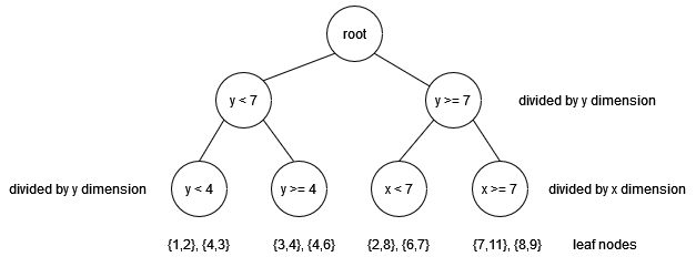
We start with a total of 8 point data where each point has two dimensions we refer to as x-dimension and y-dimension. The set of points is: {1,2}, {2,8}, {3,4}, {4,3}, {4,6}, {6,7}, {7,11} and {8,9}. Furthermore, we assume that intermediate nodes in the KDB tree can have a maximum of two children. The construction process is as follows:

The first segmentation is done on y dimension as (max_x - min_x) < (max_y - min_y) or: 7 < 9. To divide data points we first sort them according to the value of the y dimension. The result after sorting is the following list: {1,2} → {4,3} → {3,4} → {4,6} → {6,7} → {2,8} → {8,9} → {7,11}.
Then, we choose the first half of the sorted list as left subtree data and the second half of the list as right subtree data.
We continue to segment further the left subtree: now the segmentation criteria is dimension y (4 > 3). However, the segmentation criteria for the right subtree is dimension x (6 > 4). The next splitting is done in the same fashion: the data are sorted and split into left subtree and right subtree data. After this step, each intermediate node has exactly two children and the construction process stops. Finally, the KDB tree is constructed as illustrated in the figure below:

KDB tree divided by y dimension

The index file with the resulting data structure is then created as a series of blocks that contain data from leaf nodes, intermediate nodes, and the metadata of the BKD tree. The internal representation of index files is beyond the scope of this article.

Range queries¶

Numerical indexing relies on BKD tree to accelerate the performance of range queries. Considering our KDB tree, to query all points in the range x in [1,8] and y in [9,11], the engine does the following:

Starting from the root node we know from the segmentation dimension that all points where y is in [9,11] range are in the right subtree, so the next step is to traverse the right subtree.
The next segmentation dimension is the x value and from the segmentation condition, we know that points, where x is in [1,8] range, are in both left and right subtrees. So, we need to traverse both subtrees.
All child nodes of the right subtree satisfy our query range and zero child nodes from the left subtree. Finally, the query output is: {7,11} and {8,9}.

Fast sorting and aggregations¶

Document fields¶

Before Lucene 4.0, inverted indexes efficiently mapped terms to document ids but struggled with reverse lookups (document id → field value) and column-oriented retrieval. Doc values, introduced in Lucene 4.0, address this by storing field values in a column-stride format at index time, optimizing aggregations, sorting, and field access.

Lucene’s stored document fields store all field values for one document together in a row-stride fashion, and are therefore relatively slow to access.

To perform column-oriented retrieval of data, it was necessary to traverse and extract all fields that appear in the collection of documents. This can cause memory and performance issues when extracting a large amount of data from an inverted index.

Doc values¶

Doc values store data column-stride (per field), unlike stored fields which are row-stride (per document), enabling faster field-specific access, and provide fast sorting and aggregations.

Doc values is a column-based data storage built at document index time. They store all field values that are not analyzed as strings in a compact column, making it more effective for sorting and aggregations.

Because Lucene’s inverted index data structure implementation is not optimal for finding field values by given document identifier, and for performing column-oriented retrieval of data, the doc values data structure is used for those purposes instead.

Doc values allow storing numerics and timestamps (single-valued or arrays), keywords (single-valued or arrays) and binary data per row. These values are quite fast to access at search time, since they are stored column-stride such that only the value for that one field needs to be decoded per row searched.

Column store¶

CrateDB implements a column store based on doc values in Lucene. Using the Product table example:

	Document 1	Document 2	Document 3
productID	1	2	3
name	Almond Milk	Almond Flour	Milk
quantity	100	200	300

Each field’s values are stored contiguously in a column store (e.g., all productID values: 1, 2, 3), enabling efficient column-based operations.

For example, for the first document, CrateDB creates the following mappings as a column store: {productID → 1, name → “Almond Milk“, quantity → 100}.

This storage layout improves sorting, grouping, and aggregations by keeping field data together rather than scattered across documents. The column store is enabled by default in CrateDB and can be disabled for columns of type TEXT, TIMESTAMP, and all numeric data types. It does not support container or geographic data types.

Besides fields, CrateDB also supports the column store for the JSON representation of each row in a table. For this example, the row-based column store is generated as the following:

Document	Row
1	{“id”:1, “name”:”Almond Milk”, “quantity”:100}
2	{“id”:2, “name”:”Almond Flour”, “quantity”:200}
3	{“id”:3, “name”:”Milk”, “quantity”:300}

The use of a column store results in a small disk footprint, thanks to specialized compression algorithms such as delta encoding, bit packing, and GCD.

Example¶

Store data in CrateDB without the additional cost of the column store, but also without its benefits.

CREATE TABLE my_table_no_columnstore (
    str_col TEXT STORAGE WITH (columnstore = false),
    int_col INTEGER STORAGE WITH (columnstore = false),
    timestamp_col TIMESTAMP STORAGE WITH (columnstore = false),
    numeric_col NUMERIC(10, 3) STORAGE WITH (columnstore = false)
);